GEDAI spectral🔗

This tutorial demonstrates how to use spectral GEDAI. Spectral GEDAI is a frequency-specific denoising method that extends the generalized eigenvalue decomposition approach of GEDAI. Its approach focuses on isolating and removing artifacts within specific frequency bands. For that, the spectral GEDAI first decomposes the EEG data into its frequency components using wavelet transform, then applies GEDAI to each frequency band separately. Finally, the denoised frequency components are recombined to reconstruct the cleaned EEG signal.

import matplotlib.pyplot as plt
from mne.datasets import eegbci
from mne.io import concatenate_raws, read_raw_edf

from gedai import Gedai
from gedai.viz import plot_mne_style_overlay_interactive

subjects = [1]  # may vary
runs = [4, 8, 12]  # may vary
raw_fnames = eegbci.load_data(subjects, runs, update_path=True)
raws = [read_raw_edf(f, preload=True) for f in raw_fnames]
# Concatenate runs from the same subject
raw = concatenate_raws(raws)
# Make channel names follow standard conventions
eegbci.standardize(raw)

# Crop to the first 15 seconds for demonstration purposes
# (Remove or adjust this for full data analysis)
raw.crop(0, 15)
raw.pick("eeg").load_data().apply_proj()

# Apply average reference (standard preprocessing for EEG)
raw.set_eeg_reference("average", projection=False)

Extracting EDF parameters from /home/runner/mne_data/MNE-eegbci-data/files/eegmmidb/1.0.0/S001/S001R04.edf...
Setting channel info structure...
Creating raw.info structure...
Reading 0 ... 19999  =      0.000 ...   124.994 secs...
Extracting EDF parameters from /home/runner/mne_data/MNE-eegbci-data/files/eegmmidb/1.0.0/S001/S001R08.edf...
Setting channel info structure...
Creating raw.info structure...
Reading 0 ... 19999  =      0.000 ...   124.994 secs...
Extracting EDF parameters from /home/runner/mne_data/MNE-eegbci-data/files/eegmmidb/1.0.0/S001/S001R12.edf...
Setting channel info structure...
Creating raw.info structure...
Reading 0 ... 19999  =      0.000 ...   124.994 secs...
No projector specified for this dataset. Please consider the method self.add_proj.
EEG channel type selected for re-referencing
Applying average reference.
Applying a custom ('EEG',) reference.

	General
	Filename(s)	S001R04.edf
	MNE object type	RawEDF
	Measurement date	2009-08-12 at 16:15:00 UTC
	Participant	X
	Experimenter	Unknown
	Acquisition
	Duration	00:00:16 (HH:MM:SS)
	Sampling frequency	160.00 Hz
	Time points	2,401
	Channels
	EEG
	Head & sensor digitization	Not available
	Filters
	Highpass	0.00 Hz
	Lowpass	80.00 Hz

GEDAI🔗

To use spectral GEDAI, we initialize the Gedai object by specifying the wavelet_levels parameter, which defines the number of frequency bands to decompose the EEG data into. Each level corresponds to a specific frequency band, allowing for targeted denoising within those bands. It is also possible to define the type of wavelet used for the decomposition by setting the wavelet_type parameter.

gedai = Gedai(wavelet_type='haar', wavelet_level=5)

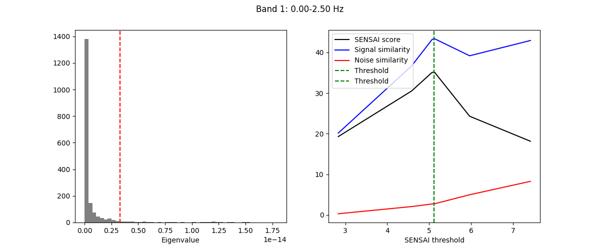
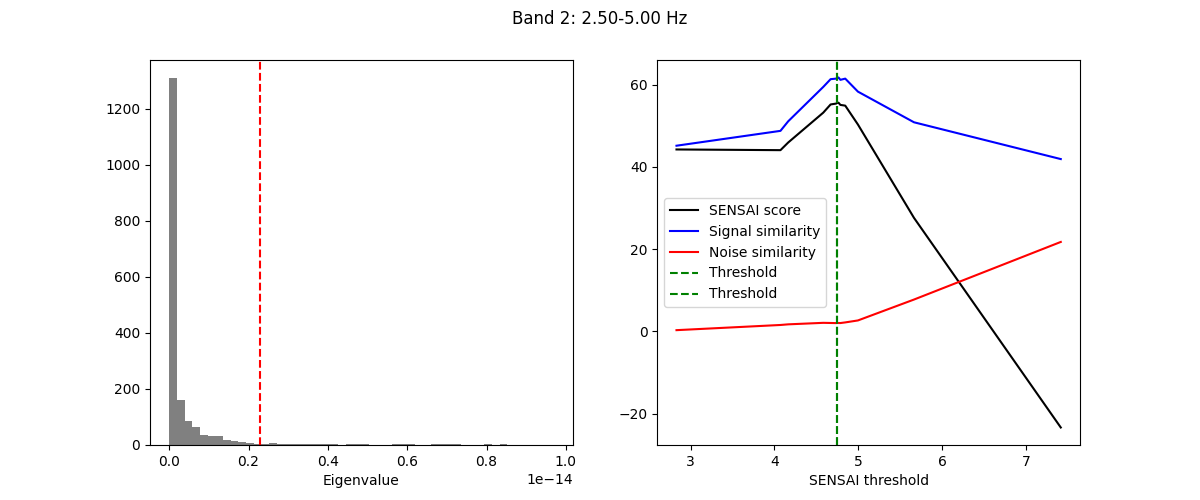
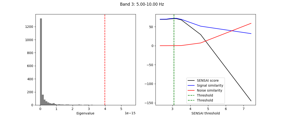
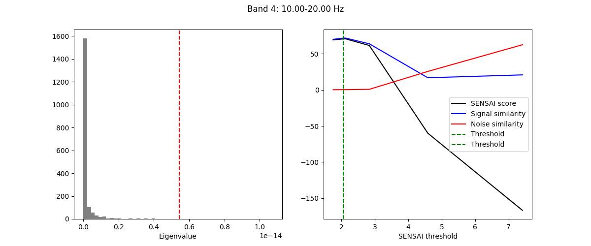
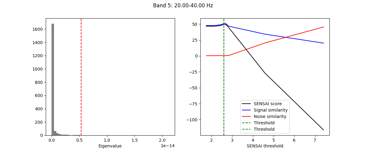
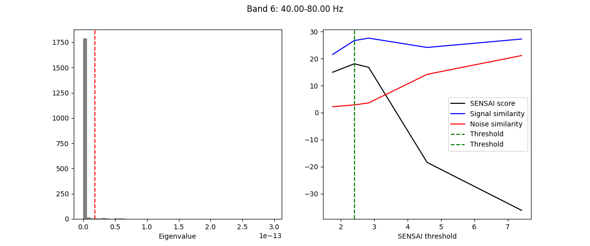
Model Fitting🔗

The fitting process of spectral GEDAI is similar to that of the standard GEDAI. For each wavelet level (i.e., frequency band), the fitting process estimates the optimal threshold to distinguish between signal and noise components.

gedai.fit_raw(raw, verbose=True)

Note

Since spectral GEDAI uses spectral decomposition, the fitting process will automatically adjust the epoch duration to ensure that each epoch contains a number of samples appropriate for the wavelet decomposition.

fig = gedai.plot_fit()
plt.show()

Transform the Data (Denoising)🔗

Once fitted, the Spectral GEDAI model can be used to remove artifacts and noise from the data. The transform operation projects out the noise components while preserving the brain signals for each frequency band separately before recombining them.

raw_corrected = gedai.transform_raw(raw, verbose=False)

Warning

Since the spectral GEDAI operates on epoched data internally, some frequency content more particularly in lower frequency bands may be not be captured properly if the epoch duration is too short. On the other hand, using very long epochs may prevent to capture short transient artifacts. Setting the wavelet_low_cutoff parameter to a value of the order of 1 / epoch_duration can help mitigate this issue by excluding lower frequency bands that may not be well estimated during the fitting process.

plot_mne_style_overlay_interactive(raw, raw_corrected)

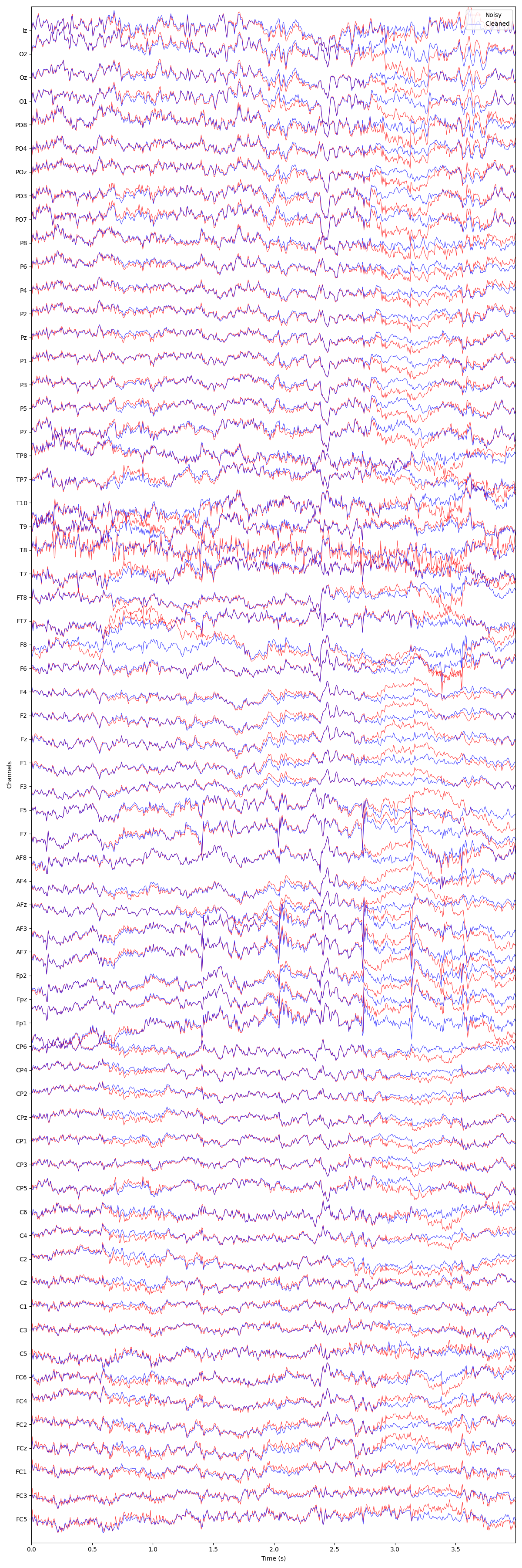
(<Figure size 1200x3600 with 1 Axes>, <Axes: xlabel='Time (s)', ylabel='Channels'>)

Recommended pipeline🔗

For optimal results, we recommend to first fit the standard GEDAI on broadband data with a conservative noise_multiplier (e.g., 6.0) to preserve most neural signals while only removing large artifacts. Then, use the resulting cleaned data to fit the spectral GEDAI model. This two-step approach leverages the strengths of both methods, ensuring effective artifact removal while maintaining the integrity of neural signals across different frequency bands.

gedai_broadband = Gedai()
gedai_broadband.fit_raw(raw, noise_multiplier=6.0)
raw_broadband_corrected = gedai_broadband.transform_raw(raw, verbose=False)

gedai_spectral = Gedai(wavelet_type='haar', wavelet_level=5, wavelet_low_cutoff=2)
gedai_spectral.fit_raw(raw_broadband_corrected, noise_multiplier=3.0)
raw_spectral_corrected = gedai_spectral.transform_raw(raw_broadband_corrected, verbose=False)

plot_mne_style_overlay_interactive(raw, raw_spectral_corrected)

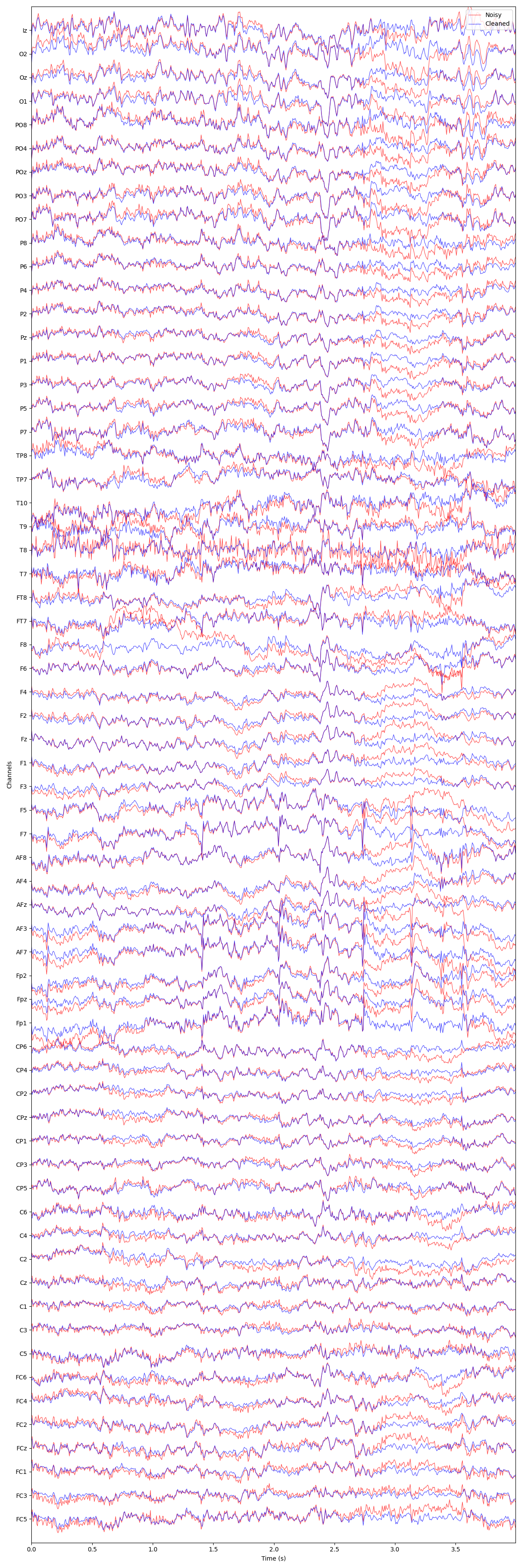
(<Figure size 1200x3600 with 1 Axes>, <Axes: xlabel='Time (s)', ylabel='Channels'>)

Total running time of the script: (11 minutes 49.126 seconds)

Estimated memory usage: 273 MB

Gallery generated by Sphinx-Gallery