Recommended Offline EEG Denoising Pipeline

This tutorial provides a practical, end-to-end offline denoising workflow using Adaptive Multiband GEDAI on EEG data.

The pipeline applies AdaptiveMultibandGedai with integrated broadband pre-cleaning:

1. Initial broadband GEDAI pass to remove gross artifacts.

2. Wavelet decomposition into adaptive frequency bands.

3. Band-specific SENSAI optimization and seamless cosine-overlap reconstruction.

Use this tutorial as a template and adapt only the data-loading block and parameter values for your own dataset.

from mne.io import read_raw

from gedai import AdaptiveMultibandGedai
from gedai.data import get_contaminated_eeg_set_path
from gedai.viz import plot_mne_style_overlay_interactive

raw = read_raw(str(get_contaminated_eeg_set_path()), preload=True)

Preprocessing GEDAI will automatically apply an average reference before fitting or transforming the data. If your acquisition used a different reference, consider adding the missing reference channel beforehand to preserve the rank of your data. For example, if your data was recorded with a Cz reference, you can add a virtual Cz channel as follows: raw.add_reference_channels("Cz", copy=False).

High-pass filtering before GEDAI usually improves covariance estimation by reducing slow drifts and non-stationarities.

raw.filter(l_freq=0.5, h_freq=None)

Filtering raw data in 1 contiguous segment
Setting up high-pass filter at 0.5 Hz

FIR filter parameters
---------------------
Designing a one-pass, zero-phase, non-causal highpass filter:
- Windowed time-domain design (firwin) method
- Hamming window with 0.0194 passband ripple and 53 dB stopband attenuation
- Lower passband edge: 0.50
- Lower transition bandwidth: 0.50 Hz (-6 dB cutoff frequency: 0.25 Hz)
- Filter length: 1321 samples (6.605 s)

	General
	Filename(s)	SNR=0.35481 contamination=25 clean_EEG_dataset_2.set + EOG_EMG_NOISE_dataset_1.set
	MNE object type	RawEEGLAB
	Measurement date	Unknown
	Participant	Unknown
	Experimenter	Unknown
	Acquisition
	Duration	00:01:00 (HH:MM:SS)
	Sampling frequency	200.00 Hz
	Time points	12,000
	Channels
	EEG	27
	Head & sensor digitization	30 points
	Filters
	Highpass	0.50 Hz
	Lowpass	100.00 Hz

Adaptive Multiband GEDAI Pipeline

We initialize AdaptiveMultibandGedai. By default, broadband_pass=True runs an initial broadband GEDAI pre-pass to remove gross artifacts before decomposing the signal into adaptive wavelet bands.

ad = AdaptiveMultibandGedai(
    wavelet_type="haar",
    wavelet_level="auto",
    cycles_per_wavelet=10,
    broadband_pass=True,
)

# Fit the model (using continuous scalar optimization by default)
ad.fit_raw(raw, noise_multiplier=3.0)

# Denoise the data
denoised_raw = ad.transform_raw(raw, verbose=False)

    343 x 343 full covariance (kind = 1) found.
[adaptive.fit_raw] INFO: Applying wavelet HP pre-filter (sub-0.50 Hz) and running broadband GEDAI pass...

Since GEDAI algorithm automatically set the reference to average, you can reset the reference to the original channel after denoising to preserve the original reference scheme: denoised_raw.set_eeg_reference(ref_channels="Cz", copy=False)

Visualize the results

plot_mne_style_overlay_interactive(raw, denoised_raw, duration=15.0)

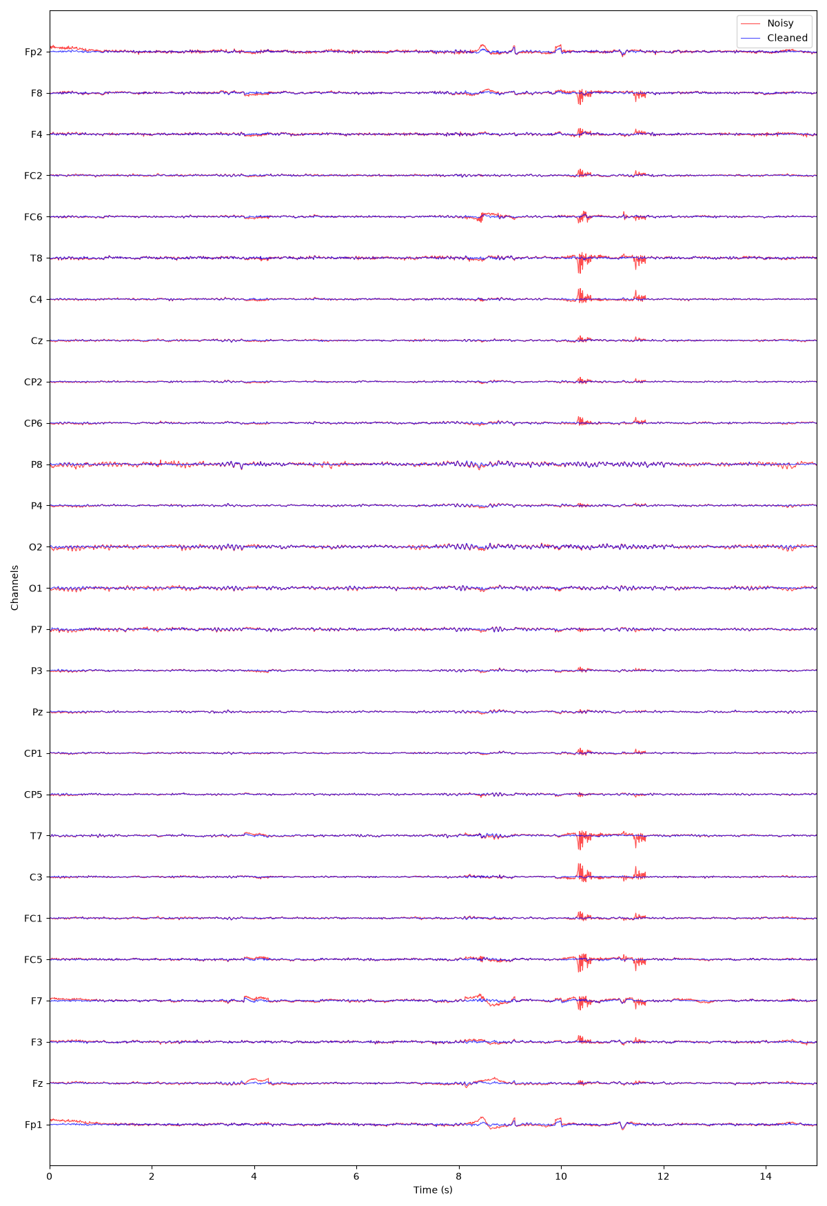
(<Figure size 1200x1750 with 1 Axes>, <Axes: xlabel='Time (s)', ylabel='Channels'>)

SENSAI Subspace Similarity & Manifold Visualization

We can evaluate and visualize the quality of the denoising using the SENSAI subspace projection. This displays the side-by-side Before/After subspace similarity projections, LDA decision boundary shading between signal and noise manifolds, and marginal distributions.

The SENSAI figure summarizes how effectively GEDAI separated genuine brain activity (signal) from artifacts (noise) by comparing the spatial patterns of the epoched data to a theoretical brain model.

Each plotted point represents a 1-second epoch in the original data (left panel), the denoised data (right panel, green points) and the removed noise (right panel, red dots).

The Axes:

• Y-axis (SSI - Subspace Similarity Index): This measures how closely the spatial topography of an epoch matches the theoretical brain model (the BEM leadfield). A value closer to 1.0 (marked by the dashed yellow line) indicates the activity is highly likely to be originating from the brain.

• X-axis (Epoch Power in dB): This represents the amplitude or strength of the signal in that specific time window. Artifacts often (but not always) have higher power than resting brain activity.

Panels:

• Left Panel (Before Denoising): This displays your raw EEG epochs prior to cleaning. The color gradient corresponds to the SSI score (yellow/green is more brain-like, blue/purple is less brain-like). You will typically see a wide spread of data here, where epochs with high power and low SSI are clear indicators of prominent, non-brain artifacts (like blinks or gross muscle movement).

• Right Panel (After Denoising): This illustrates the core separation achieved by the algorithm, dividing the data into two distinct clusters (along with density distribution curves on the top and right borders):

  • Green dots (Signal): These are the components GEDAI identified as genuine brain activity and kept. Notice how they cluster tightly near the 1.0 line, indicating high spatial similarity to the brain leadfield.

  • Red dots (Noise): These are the artifact components GEDAI removed. They generally exhibit lower similarity to the brain leadfield and are often scattered across a wider range of power levels.

Sub-optimal Denoising Outcomes:

• Noise-in-the-Signal: The Red (Noise) cluster contains some Green (Signal) dots (i.e. under-cleaning, “noise” components were missclassified as “signal”).

• Signal-in-the-Noise: The Green (Signal) cluster contains some Red (Noise) dots (i.e. over-cleaning, “signal” components were missclassified as “noise”).

Key Metrics:

• SSI Silhouette Score: This is a clustering metric that evaluates how cleanly separated the “Signal” (green) and “Noise” (red) groups are along the SSI axis. A score close to 1.0 (e.g., 0.97) represents excellent, distinct separation, meaning the algorithm confidently isolated artifacts from brain signals.

• Mean SSSI (Signal Subspace Similarity Index): The average similarity score of the retained brain data (you want this to be high).

• Mean NSSI (Noise Subspace Similarity Index): The average similarity score of the rejected artifact data (you generally expect this to be much lower than the SSSI).

fig, metrics = ad.plot_sensai(raw_before=raw, raw_after=denoised_raw)

Estimated memory usage: 316 MB