Note
Go to the end to download the full example code.
Understanding the adaptive extension of multiband GEDAI🔗
This tutorial demonstrates how to use Adaptive Multiband GEDAI.
The method tackles the limitations of the standard multiband GEDAI
by automatically determining the optimal epoch duration for each
band (i.e., wavelet level) based on the frequency content of the band.
By doing so, it allows to capture both transient and sustained artifacts
across different frequency ranges.
Note
This purpose of this tutorial is to explain the differrent parameters of
the AdaptiveMultibandGedai model and help you
better understand the underlying algorithm. If you want to learn how to
use Adaptive Multiband GEDAI in a practical, end-to-end offline
denoising workflow, please refer to the
Practical Pipelines section.
For simplicity, we will only use the first 30 seconds of the data in this tutorial. In practice, it is recommended to use the full recording for fitting the GEDAI model, as this allows the model to better capture the noise characteristics of the data.
raw.crop(0, 30)
Before using the AdaptiveMultibandGedai model,
it is recommended to first apply the broadband Gedai model
to remove large artifacts while preserving most of the neural signals.
For that, we use a conservative noise_multiplier (e.g., 6.0) to
ensure that only the most extreme artifacts are removed.
broadband_gedai = Gedai()
broadband_gedai.fit_raw(raw, noise_multiplier=6.0, n_jobs=n_jobs, verbose=False)
broadband_denoised_raw = broadband_gedai.transform_raw(
    raw, n_jobs=n_jobs, verbose=False
)
GEDAI Adaptive Multiband model🔗
The AdaptiveMultibandGedai model uses wavelet decomposition to
separate the EEG data into different frequency bands and applies GEDAI
separately to each band.
The wavelet decomposition is controlled by the
- wavelet_type
- wavelet_level parameters.
%%
The wavelet type (wavelet_type) can be any wavelet supported by the
PyWavelets library (e.g., haar, db4, etc.). The default type haar
works well in most cases and is computationally efficient.
wavelet_type = "haar"
The wavelet level (wavelet_level) controls the number of frequency
bands that the data is decomposed into.
The optimal level depends on the sampling frequency. Typically, users should
choose a level that provides good coverage of the classical EEG frequency
bands (e.g., delta, theta, alpha, beta, gamma).
For example, for a sampling frequency of 200 Hz, a wavelet level of 9
provides wavelet bands with the following frequency ranges:
(0.00 - 0.20 Hz)
(0.20 - 0.39 Hz)
(0.39 - 0.78 Hz)
(0.78 - 1.56 Hz)
(1.56-3.12 Hz) Delta
(3.12-6.25 Hz) Theta
(6.25-12.5 Hz) Alpha
(12.5-25 Hz) Beta
(25-50 Hz) Gamma
(50-100 Hz) High Gamma
(100-200 Hz)
wavelet_level = 9
For each wavelet level, AdaptiveMultibandGedai will automatically
determine the optimal epoch duration. Slower frequency bands will be
estimated on longer epochs, while faster frequency bands will be estimated on
shorter epochs.
This adaptive approach allows both transient and sustained artifacts to be
captured across different frequency ranges.
The cycles_per_wavelet parameter controls the number of cycles of the
wavelet that are included in each epoch. Higher values lead to longer epochs,
while lower values lead to shorter epochs. A minimum of 2 cycles per wavelet
is recommended to ensure proper estimation of the covariance matrix.
cycles_per_wavelet = 10
With these parameters defined, we can now instanciate the model:
adaptive_multiband_gedai = AdaptiveMultibandGedai(
    wavelet_type=wavelet_type,
    wavelet_level=wavelet_level,
    cycles_per_wavelet=cycles_per_wavelet,
)
The fitting process of AdaptiveMultibandGedai is similar to that of the standard
Gedai. The main difference is that the fitting process
is performed separately for each wavelet level (i.e., frequency band).
As seen previously, some wavelet levels contain very low frequencies. This
frequency content would require very long epochs to be properly estimated.
In addition, these frequency bands often fall below the high-pass filter
cutoff frequency and therefore do not contain meaningful information. To
mitigate this issue, the additional wavelet_low_cutoff parameter controls
which wavelet levels (i.e., frequency bands) should be ignored.
Frequency bands with an upper cutoff frequency below the specified
wavelet_low_cutoff will be automatically ignored during the fitting and
transformation process.
When set to auto, wavelet_low_cutoff will be automatically set to the
highest value between raw.info[‘highpass’] and the upper frequency cutoff of
the slowest wavelet level.
When set to a value, wavelet_low_cutoff will be set to the specified
value. This can be useful when the user wants to exclude more wavelet levels
than the default auto setting. However, it is not advised to set this
parameter below the upper frequency cutoff of the slowest wavelet level.
Note
When loading data from a different format than .fif, MNE may not be
able to automatically load info['highpass'] and will set it to 0.0
by default. If you know the high-pass filter cutoff frequency that was
applied during acquisition or preprocessing and this value is above the
upper frequency cutoff of the slowest wavelet level, it is recommended to
set the wavelet_low_cutoff parameter to this value to ensure that
low-frequency wavelet levels are properly ignored during the fitting and
transformation process.
# In the current example, the upper frequency cutoff of the slowest wavelet
# level is around 0.2 Hz while the high-pass filter cutoff is at 0.5 Hz.
# Therefore, the ``auto`` setting will lead to a ``wavelet_low_cutoff`` of 0.5
# Hz, which will result in excluding the (0.00 - 0.20 Hz) and (0.20 - 0.39
# Hz) wavelet levels from the fitting and transformation process.

wavelet_low_cutoff = "auto"
a stronger noise multiplier (e.g., 3.0) can be used to give more weight
to noise removal.
noise_multiplier = 3.0
We fit the model on the broadband-denoised data.
adaptive_multiband_gedai.fit_raw(
    broadband_denoised_raw,
    noise_multiplier=noise_multiplier,
    wavelet_low_cutoff=wavelet_low_cutoff,
    n_jobs=n_jobs,
)
The different wavelet parameters are stored in the
adaptive_multiband_gedai._wavelets_fits attribute. The ignore key
indicates which wavelet levels were ignored based on the
wavelet_low_cutoff setting. The duration key indicates the epoch
duration used to estimate the GEDAI model of the corresponding wavelet
level.
[{'band_index': 0, 'fmin': 0.0, 'fmax': 0.1953125, 'model': None, 'duration': None, 'n_samples': None, 'ignore': True}, {'band_index': 1, 'fmin': 0.1953125, 'fmax': 0.390625, 'model': None, 'duration': 51.2, 'n_samples': 10240, 'ignore': True}, {'band_index': 2, 'fmin': 0.390625, 'fmax': 0.78125, 'model': <gedai.gedai.gedai.Gedai object at 0x7f03589f2950>, 'duration': 25.6, 'n_samples': 5120, 'ignore': False}, {'band_index': 3, 'fmin': 0.78125, 'fmax': 1.5625, 'model': <gedai.gedai.gedai.Gedai object at 0x7f0358316cd0>, 'duration': 12.8, 'n_samples': 2560, 'ignore': False}, {'band_index': 4, 'fmin': 1.5625, 'fmax': 3.125, 'model': <gedai.gedai.gedai.Gedai object at 0x7f035874b750>, 'duration': 7.68, 'n_samples': 1536, 'ignore': False}, {'band_index': 5, 'fmin': 3.125, 'fmax': 6.25, 'model': <gedai.gedai.gedai.Gedai object at 0x7f0349fe2150>, 'duration': 5.12, 'n_samples': 1024, 'ignore': False}, {'band_index': 6, 'fmin': 6.25, 'fmax': 12.5, 'model': <gedai.gedai.gedai.Gedai object at 0x7f0386477190>, 'duration': 5.12, 'n_samples': 1024, 'ignore': False}, {'band_index': 7, 'fmin': 12.5, 'fmax': 25.0, 'model': <gedai.gedai.gedai.Gedai object at 0x7f03682a3290>, 'duration': 5.12, 'n_samples': 1024, 'ignore': False}, {'band_index': 8, 'fmin': 25.0, 'fmax': 50.0, 'model': <gedai.gedai.gedai.Gedai object at 0x7f03864857d0>, 'duration': 5.12, 'n_samples': 1024, 'ignore': False}, {'band_index': 9, 'fmin': 50.0, 'fmax': 100.0, 'model': <gedai.gedai.gedai.Gedai object at 0x7f0358196290>, 'duration': 5.12, 'n_samples': 1024, 'ignore': False}]
The wavelet models results can also be visualized using the plot_fit method:
adaptive_multiband_gedai.plot_fit()
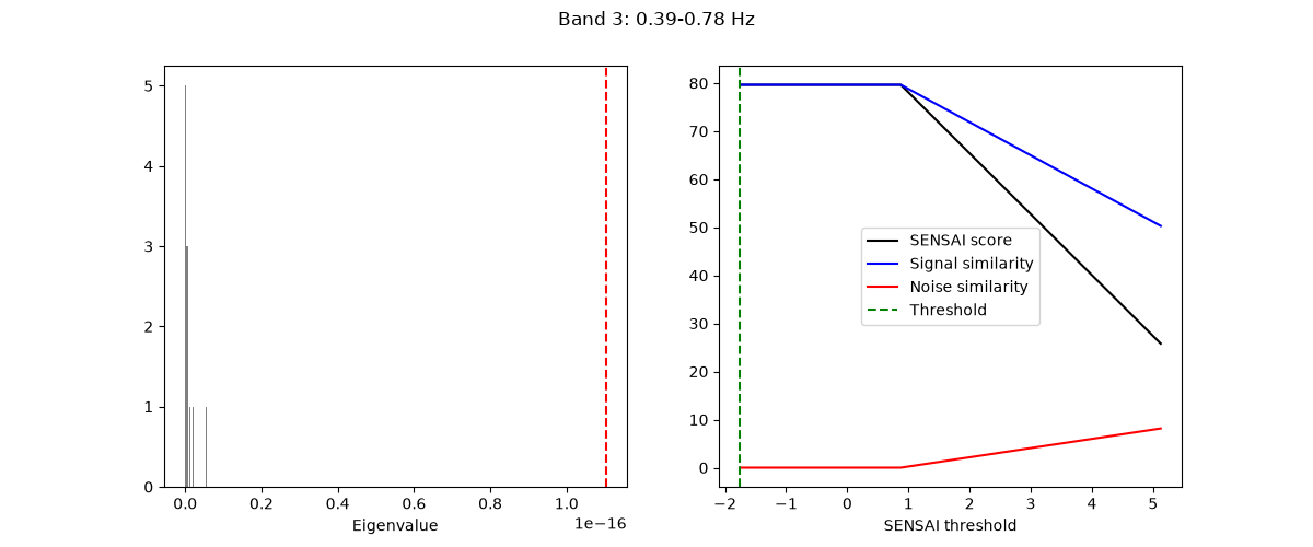
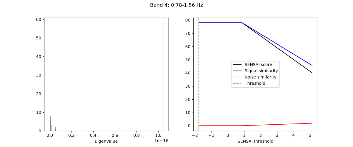
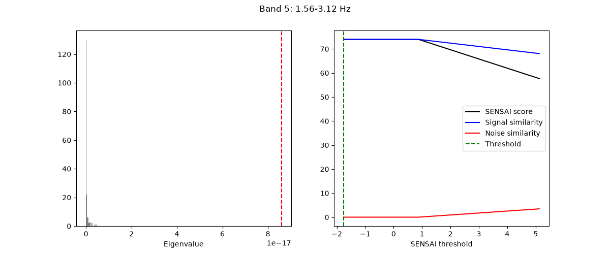
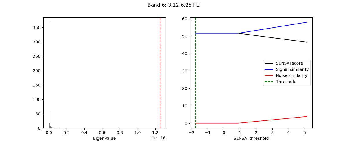
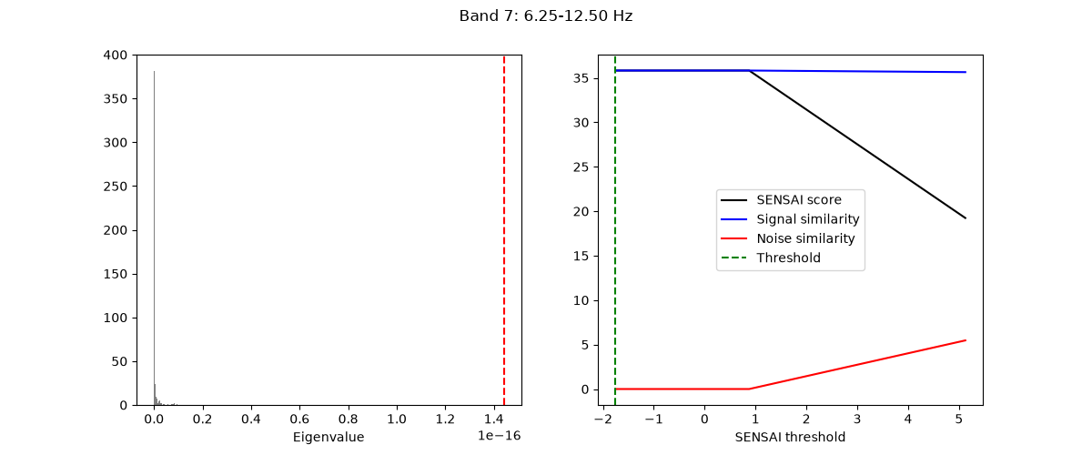
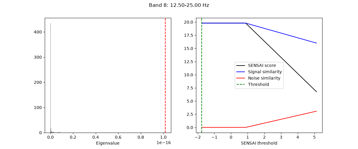
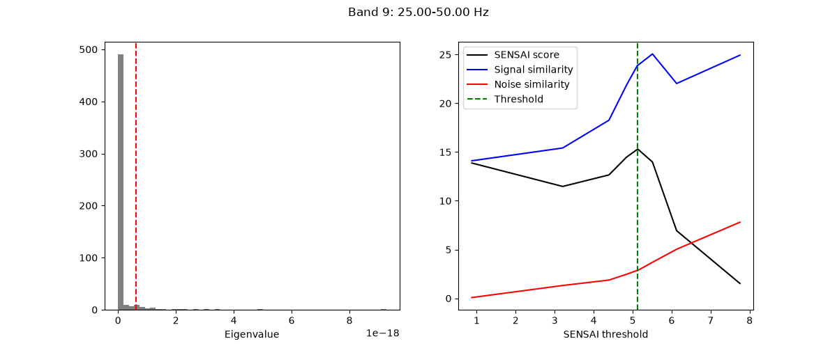
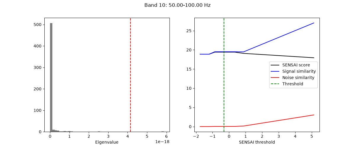
[<Figure size 1200x500 with 2 Axes>, <Figure size 1200x500 with 2 Axes>, <Figure size 1200x500 with 2 Axes>, <Figure size 1200x500 with 2 Axes>, <Figure size 1200x500 with 2 Axes>, <Figure size 1200x500 with 2 Axes>, <Figure size 1200x500 with 2 Axes>, <Figure size 1200x500 with 2 Axes>]
The model can then be used to denoise the data:
adaptive_multiband_denoised_raw = adaptive_multiband_gedai.transform_raw(
    broadband_denoised_raw, n_jobs=n_jobs
)
Finally, we can visualize the results:
plot_mne_style_overlay_interactive(raw, adaptive_multiband_denoised_raw, duration=15.0)
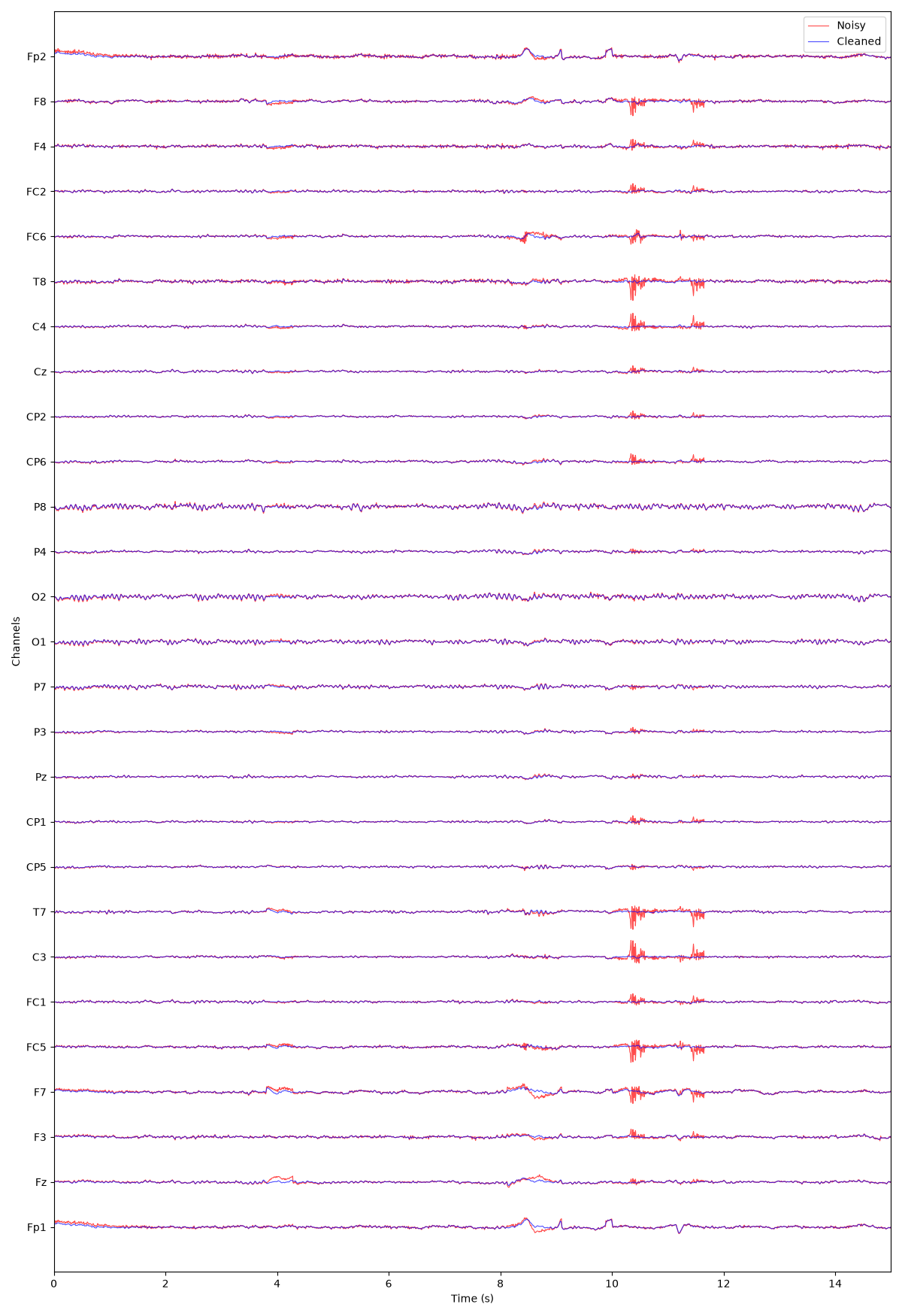
(<Figure size 1200x1750 with 1 Axes>, <Axes: xlabel='Time (s)', ylabel='Channels'>)
Total running time of the script: (5 minutes 8.707 seconds)
Estimated memory usage: 339 MB